DynamoDB

DynamoDB Accelerator (DAX)

DynamoDB is a Database as a Service (DBaaS) (RDS and Aurora are DBSaaS), o more a Table as a Service, service. It can handle Key/Value data or Document structures. There are no servers, just tables.

It’s a public service, it lies in the AWS Public Zone, so it can only be accessed within a subnet with a route to an Internet Gateway, a Nat Gateway, or a VPC Gateway Endpoint.

DynamoDB is region resilient and optionally globally resilient.

Its storage is SSD-based, so it provides single-digit millisecond access times. Also, data is encrypted at-rest.

It supports event-driven integrations with AWS services on data changes.

DynamoDB is accessible via Console, CLI, and API. There’s NO query language available (PartiQL is available though).

Tables

Tables are groupings of items that share the same Primary Key.

Primary keys can be:

Simple or Partition Key (PK)

Partition Key 1

attribute_1

attribute_2

attribute_3

attribute_4

attribute_5

attribute_6

attribute_7

attribute_8

Partition Key 1

attribute_1

attribute_2

attribute_3

attribute_4

attribute_5

attribute_6

attribute_7

attribute_8

Partition Key 1

attribute_2

attribute_3

attribute_4

attribute_5

attribute_6

attribute_7

Partition Key 1

attribute_9

Partition Key 1

attribute_12

attribute_4

attribute_25

attribute_14

attribute_7

Composite (Partition Key + Sort Key (SK)):

Partition Key 1

Sort Key 2

attribute_1

attribute_2

attribute_3

attribute_4

attribute_5

attribute_6

attribute_7

attribute_8

Partition Key 1

Sort Key 1

attribute_1

attribute_2

attribute_3

attribute_4

attribute_5

attribute_6

attribute_7

attribute_8

Partition Key 1

Sort Key 7

attribute_2

attribute_3

attribute_4

attribute_5

attribute_6

attribute_7

attribute_8

Partition Key 1

Sort Key 99

attribute_66

Partition Key 1

Sort Key 3

attribute_11

attribute_2

attribute_3

attribute_4

attribute_25

attribute_6

attribute_7

attribute_8

The combination of the partition key and the sort key must be unique in the table.

Each item in the table can have no rigid schema: they can have different attributes.

The Maximum Item size is 400 KB, including the PK and SK.

Capacity

Capacity = Compute power/units = CUs

Capacity does not refer to storage.

Capacity is set per table.

Read Capacity Unit (RCU) = 1 KB/s
Write Capacity Unit (WCU) = 4 KB/s

Reads and Writes round up to the next multiple of 1 RCU/WCU (with 1 RCU being 4 KB/s in strong consistency and 1 WCU being 1 KB/s in strong consistency): if you READ a total of 5KB, then you need 2RCUs (wasting 3KB read).

Requests per second

Reads up to 4KB:
- Strong consistency: 1 request/s = 1RCU
- Eventual consistenct: 2 requests/s = 0.5 RCUs
- Transactional: Transactional read requests require two RCUs to perform one read per second for items up to 4 KB ⇒ 2 RCUs
Writes up to 1 KB:
- Standard: 1 request/s = 1 WCU
- Transactional: Transactional write requests require two WCUs to perform one write per second for items up to 1 KB ⇒ 2 WCUs

WCU Calculation

Example: you need to store 10 items per second, 2.5 KB average size per item.

Each item: 2.5 KB == round up ⇒ 3 WCUs (1 WCU = 1 KB/S)

To sustain 10 items per second you need to provision 30 WCU capacity.

Example: retrieve 10 items per second, 2.5 KB average size per item.

Each item is 2.5 == round up ⇒ 1 RCU (1 RCU = 4 KB/s)

To sustain 10 items per second you need to provision 10 RCU capacity if you want Strong consistency.

Eventual consistency requires only 1/2 of the RCUs, so to sustain a continuous read of 10 items per second you need 5 RCUs.

On-Demand

You don’t manage capacity, you pay a cost per operation: you pay a price per milion RCUs or WCUs. The price can be as much as 5 times higher than with Provisioned mode.

Useful for unknown or unpredictable levels of load on a table, or for minimizing admin overhead.

You can switch a newly created table in on-demand mode to provisioned capacity mode at any time. However, you can only switch it back to on-demand mode 24 hours after the table’s creation timestamp or 24 hours after the last timestamp indicating a switch to on-demand

Provisioned

You set the capacity per table in terms of RCUs and WCUs. But you can use Auto Scaling to adjust your table’s provisioned capacity automatically in response to traffic changes.

In this mode every table has a RCU and WCU burst pool of 300 seconds.

On-demand mode supports up to 4,000 writes per second and 12,000 reads per second. If your workload generates more than double your previous peak on a table, DynamoDB automatically allocates more capacity as your traffic volume increases. However, throttling can occur if you exceed double your previous peak within 30 minutes.

Operations

Every READ operation on a Table consumes AT LEAST (even if no result is returned):

0.5 RCU for Eventually Consistent Reads
1 RCU for Strongly Consisten Reads
2 RCUs for Transactional reads

Table 1. Example table: Artist is the PK and Album the SK
artist	album	title	bitrate	track_n
Shantel	Disko Partizani	Disko Partizani	320	4
Shantel	Disko Partizani	Disko Boy	320	2
Shantel	Shantology	Gas Gas Gas	256	9
Caro Emerald	Deleted Scenes From the Cutting Room Floor	The Other Woman	320	5
Unknown	-	La-la-song	-	-

Let’s say that the first record (title: Disko Partizani) is 1 KB in size.
The second record (title: Disko Boy) is 0.8KB
The third record (title: Gas Gas Gas) is 1 KB
The fourth record is (title: the other woman) 2 KB
The fifth record is (title: La-la-song) 0.5 KB

Query

You can query data by:

Partition Key (PK)
Partition Key + Sort Key (SK)

You can only query for a single PK or PK + a condition for the SK. Valid queries in the example table would be:

pk=Shantel
pk=Shantel,sk="Disko Partizani"
pk=Shantel,sk=begins_with('Disko ')

Available operators for the SK: = > < >= ⇐ BETWEEN-AND begins_with

Thhe pk=Shantel,sk="Disko Partizani" query would return:

artist

album

title

bitrate

track_n

Shantel

Disko Partizani

320

Shantel

Disko Partizani

Disko Boy

320

If you don’t specify filters you get all the matching items, RCUs consumed are the sum of the sizes for all items.

The resulting compute requires is (1 + 0.8) KB read in 1 sec = 1.8 KB read in 1 sec == round up ⇒ 4KB ⇒ 1 RCU

If you apply filters you are billed for the same: pk=Shantel,sk="Disko Partizani",filter=title is still 1 RCU.

If nothing matches only 0.5 RCUs are consumed for an Eventually Consistent read or 1 RCU for a Strongly Consistent read.

In terms of efficiency it’s always more efficient to query for multiple items rather than a specific one per operation because of the round up.

Scan

Scan is more flexible but more expensive. You can match any attributes, not just the keys, not just the PK and the SK.

Scan will scan the entire table! You’ll consume as many RCUs as needed to return the whole table!

Example: Scan(bitrate=320)

artist

album

title

bitrate

track_n

Shantel

Disko Partizani

320

Shantel

Disko Partizani

Disko Boy

320

Caro Emerald

Deleted Scenes From the Cutting Room Floor

The Other Woman

320

You’ll consume the sum of:

title: Disko Partizani (1 KB)
title: Disko Boy (0.8 KB)
title: Gas Gas Gas (1 KB) ⇐ [.underline]#even if this item is not returned because it doesn’t match! It has a 256 Kbps bitrate.
title: The Other Woman (2 KB)
title: La-la-song (0.5 KB)

Which is 1 + 0.8 + 1 + 2 + 0.5 = 5.3 KB/s == round up ⇒ 2 RCUs (1 RCU is 4.0 KB/s)

Consistency

DynamoDB Tables are regional (they can also be global). You have one node in each availability zone or so.

When you write data you write to the elected leader node, changes are then replicated across all nodes (milliseconds), but if you happen to read while data replication is not complete you might get an inconsisten result because DynamoDB directs you to one of the nodes at random.

You can choose to perform Eventually consisten reads or Strongly consistent reads: the former expose you to the risk of getting an inconsistent result but require less RCUs, the latter guarantee you a consistent result but at the cost of more RCUs. Strongly consistent reads are directed to the leader node, so data is always updated because that’s the node you write to.

You can choose between these two modes but if you choose eventual consistency your application needs to support it.

Transactions

With transactions you group reads or writes and submit them as an all-or-nothing operation.

You can read using the TransactGetItems API.

You can write using the TransactWriteItems API, and you can optionally include a client token to make the operation idempotent in case of a repeated transaction due to network issues.

Secondary Indexes

Secondary indexes allow for alternate views of data and more efficient data retrieval using alternative access patterns if well planned.

They allow to specify an alternate Sort Key (LSIs) or an alternate Primary Key and sort Key (GSIs) and to choose what other attributes to project (less data to return) in the secondary index.

Indexes are SPARSE INDEXES: only items from the base table that actually HAVE a value for the secondary index Sort Key are included in the secondary index. The unknown artist will not be included in an index where 'bitrate' is the PK/SK because the value for bitrate is not present in the base table.

This means:

Secondary indexes act like queries, optionally with filters: if you know you’ll make always the same query it’s more efficient to create a secondary index insted.
You can now scan the secondary index knowing that only items containing a value for the secondary index keys will be scanned, NOT the whole base table

As a generar rule you should default to GSIs, and only use LSIs only if Strong Consistency is required.

Local Secondary Indexes (LSIs)

You can specify an alternate Sort Key, more convenient for the view you want to build, but you must use the same Partition Key. Local Secondary Indexes MUST be created WHEN THE BASE TABLE IS CREATED. You can’t add LSIs to an existing table.

You can create up to 5 per base table.

Read and Write capacity is SHARED with the base table.

With LSIs you can have both STRONG and EVENTUAL consistency.

As far as including attributes is concerned, you can choose to include:

All attributes
Keys only, the Partition Key and the Sort Key
A subset of attributes

Table 2. Example Local Secondary Index: 'bitrate' becomes the SK, 'artist' remains the PK
artist	bitrate	title
Shantel	320	Disko Partizani
Shantel	320	Disko Boy
Shantel	256	Gas Gas Gas
Caro Emerald	320	The Other Woman

La-la Song is not included because it has no value for bitrate, the SK for this LSI.

Now I can query for bitrate without having to perform a scan!

If you query or scan a local secondary index, you can request attributes that are not projected in to the index, DynamoDB automatically fetches those attributes from the table, but it’s extremely inefficient.

Global Secondary Indexes (GSIs)

Global Secondary Indexes are similar to Local ones but:

You can set both the PK and OPTIONALLY SK to any attribute
You can create them whenever you need one, not just on base table creation
They only allow EVENTUAL CONSISTENCY because data is replicated from the base table to the GSI asynchronously.
They have an independent RCU/WCU allocation from the base table.
You can have up to 20 per table

As far as including attributes is concerned, you can choose to include:

All attributes
Keys only, the Partition Key and the Sort Key
A subset of attributes

With global secondary index queries or scans, you can only request the attributes that are projected into the index. DynamoDB does not fetch any attributes from the table.

Event-Driven Integration

DynamoDB Streams captures a time-ordered sequence of item-level modifications in any DynamoDB table and stores this information in a log for up to 24 hours (24 hours rolling window). Applications can access this log and view the data items as they appeared before and after they were modified, in near-real time.

Each stream record appears exactly once in the stream and the stream records appear in the same sequence as the actual modifications to the item.

Streams endpoint: streams.dynamodb.<region>.amazonaws.com

Streams need to be explicitly enabled on a table and you can use:

DynamoDB Streams
Kinesis Data Streams for extended capabilities and up to 1 year retention.

Records in a table are generated for the following operations:

Create
Delete
Update

And for each stream you can set the content of the record by setting the View Type:

KEYS_ONLY — Only the key attributes of the modified item.
NEW_IMAGE — The entire item, as it appears after it was modified. Useful for further processing the new/updated item without having to query.
OLD_IMAGE — The entire item, as it appeared before it was modified. Useful for backing up.
NEW_AND_OLD_IMAGES — Both the new and the old images of the item. Useful for comparing.

For newly created items, if the NEW_AND_OLD_IMAGES is used, the old value will be empty, same for deleted objects using NEW_IMAGE or NEW_AND_OLD_IMAGES, and so on…

They allow for a Database Triggers architecture in a serverless way: a Lambda Function can be invoked for each record.

Use Cases

Reporting
Analytics
Aggregation
Messaging and Notification

See DynamoDB Streams Use Cases and Design Patterns.

Global Tables

This feature provides multi-master write (active-active setup) replication of DynamoDB tables #across multiple AWS Regions.

You create tables in different regions and in one table you configure the links between all tables.

You can write to all the regions involved and conflict resolution uses last-writer-wins

Replication happens in < 1s between region but you only get both STRONG AND EVENTUAL consistency in the region where the write happens, in all other regions you get EVENTUAL consistency ONLY.

Use Cases

Global High Availability
Global Disaster Recovery
Global Business Continuity

DynamoDB TTL

Sets an expiration per item expressed in seconds since the EPOCH.

It’s set using an attribute of the item that contains the timestamp and then marking that attribute as the TTL container.

Automated processes run on the table:

A per partition process scans the table and only marks items as expired.
Another per partition process deletes the marked items from the table and from any indexes and also adds the deletion to any configured streams.

These processes run in the background and do not consume capacity or add additional charges.

Also, a dedicated TTL Deletion Stream can be enabled, where all these deletions converge.

For example you may want to retain some data and write an undelete function that the TTL Delete stream invokes each time and that decides if the item should go back or stay deleted.

Backups

On-Demand

They’re performed manually, they’re not initiated automatically by AWS.

Similarly to RDS snapshots:

Retained until you delete them: their lifecycle is in your hands.
They’re a full copy of a table.

Restore

They can be restored (with or without indexes) to the same region or cross-region.

Upon restore you can also adjust encryption settings.

Point-In-Time Recovery

It’s a continuous backup flow and it’s disabled by default.

Backups of this kind allow to go back in time with 1 second granularity (!!) over a 35 days retention period (Recovery Window).

You can also create a table restoring from a point in time.

DynamoDB example architecturees

Mobile Applications

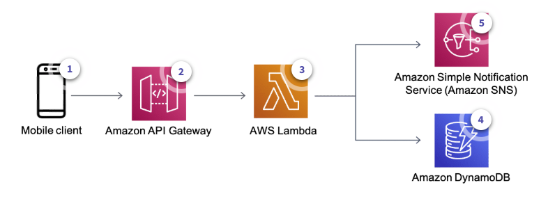
The user updates their status
API Gateway gets the request and invokes a Lambda function
The Lambda function:
1. Looks up the friends list of that user
2. Uses SNS to send a push notification to the user’s friends

Anomaly Detection

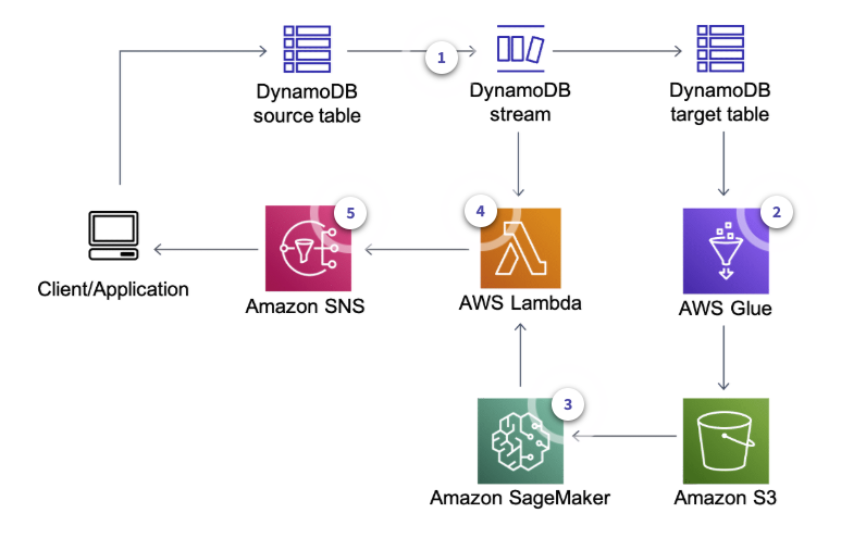
Figure 1. See Anomaly detection on Amazon DynamoDB Streams using the Amazon SageMaker Random Cut Forest algorithm for details

Wneh a user makes a change DynamoDB captures a change and stores it in a DynamoDB Stream
AWS Glue job regularly retrieves data from target DynamoDB table and runs a training job using Amazon SageMaker to create or update model artifacts on Amazon S3
The same AWS Glue job deploys the updated model on the Amazon SageMaker endpoint for real-time anomaly detection based on Random Cut Forest
AWS Lambda function polls data from the DynamoDB stream and invokes the Amazon SageMaker endpoint to get inferences
The Lambda function alerts user applications after anomalies are detected

Billing

It’s based on:

Capacity or Operations (depending on the capacity mode)
Storage
Enabled features